As a whole, Canadians have a good quality of life and enjoy healthy incomes, most of which comes from employment income. However, government transfer payments play an important role in the Canadian economy when one considers unemployment benefits, family allowance payments, welfare, and G.S.T. rebates. Regional differences also affect the economic climate in Canada, causing variations in personal income per capita among the provinces, and differences in government transfer payments. For example, Ontario is the most populous province, is industry-based, and is home to the headquarters of many Canadian corporations. It has some of the highest incomes per capita when compared with the other provinces. Would it be true to say that as Ontario's employment incomes increase, its government subsidies decrease? Or, that as employment incomes decrease, government subsidies increase? Take Newfoundland, for example. When the fishery was collapsing and the fisherpeople were told they had to wait until fish stocks increased before working again, was there a correlating increase in government subsidies? Of course there was, because many people went on welfare after their unemployment insurance ran out, or applied for retraining programs that were being offered. This report will examine if this correlation exists between employment income and government sources in the Canadian economy, and endeavour to make some interpretations and predictions based on the data.
This study is investigating the relationship between two variables: 1.) percentage of total income from wages and salaries, and, 2.) percentage of total income from government sources, to establish if there is a significant correlation between them. It is using a stratified sample of Canadian provinces and territories taken from the 1991 Census data. The sampling unit is census division (county). The null hypothesis states that there is no significant correlation between the percentage of total employment income and the percentage of total income from government sources in the Canadian population. The alternative hypothesis states that there is a significant correlation between the percentage of total employment income and the percentage of total income from government sources in the Canadian population.
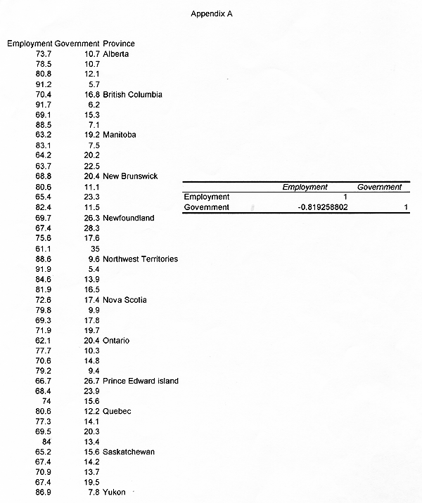
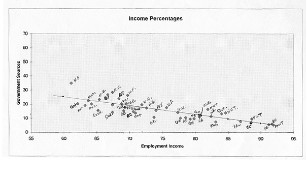
To begin the bivariate analysis, the first step is to construct a scattergram to illustrate the relationship. Each dot represents a paired value from the sample. The scattergram reveals a typical oval shape that is due to central tendency (Sprinthall 1990,200). Clearly, there seems to be a fairly strong relationship in the sample between the two variables, one that it is linear and negative (See Appendix C). There is a strong negative relationship, which means that as the percentage of total employment income increases, the percentage of total income from government sources decreases, and inversely, as employment income decreases, income from government sources increases. To find out how strong the correlation actually is requires a statistical measure. The Product-Moment Correlation Coefficient, or Pearson's Correlation Coefficient allows the researcher to express "the relationship between two qualitatively different objects in quantitative terms" (Sprinthall 1990,196). The result or 'r-value' is -0.819 (-0.819258802, see Appendix A). By checking it against the critical value, which is approximately .300 at a confidence level of 95%, the Pearson's r is greater. Therefore, the null hypothesis is rejected, since there is enough evidence to say that the two variables are related. Because the coefficient is so strong, we can infer that there is a real relationship between them in the population.
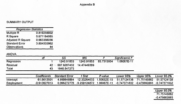
In the social sciences, the basic reason for doing statistical analysis is to uncover trends, reveal relationships, and to make predictions. Regression analysis allows social scientists to make predictions, using knowledge of the independent variable (Walsh 1990,260). To do this, a linear equation or regression equation is needed to plot a regression line. Since there is a linear relationship, a straight line can be fitted to the data and used for prediction. The regression equation is used because "it is said to be the best estimator of the linear model, [and] on the whole it yields the smallest residuals" (O'Sullivan 1995,417). Using the model y = a + bx, regression analysis will be run on Excel to find the values for a and b. Results are found in Appendix B, and give a value of 61.66 for a (intercept), and -0.6136 for b (slope). Therefore, y = 61.66 + (-0.6136 multiplied by x). By choosing x values from both ends of the axis, two dots can be inserted and connected to form the line (See Appendix C).
This line is the one that best describes the income percentage data. Predictions can now be made based on the regression line. Even though we do not live in a perfect world and cannot make perfect predictions, it is still important that we try to forecast trends in the future, and develop contingency plans based on data extrapolation. Caution is the maxim for predictions. For example, if we wanted to predict the percentage of total income from government sources for a county with 85 percent income from wages and salaries, we can do so, and it will be close to 9.50 percent. What this means is that regression can help to predict one variable based on another if they are related to each other, as changes in a variable x are thought to explain changes in another variable y. More importantly, it can "infer population characteristics based on a sample" (O'Sullivan 1995,414). For this data analysis, the coefficient of determination is .6712, meaning that 67% of the variability in the percentage of total income from government sources can be explained by variability in the percentage of total income from wages and salaries. The larger the coefficient of determination, the more accurate the predictions will be. In this case, it is only one of the variables affecting the percentage of government transfer payments; 33% of the variability in y must be explained by other factors (Rowntree 1991,173).
The regression model can be used to indicate how well Canadian provinces are actually doing economically when compared with each other. If it's true that government sources drop as employment income increases, the federal government may begin looking at particular provincial economies to decide whether job creation programs would help to raise employment figures, and, as a result, lower government transfer payments. It may decide that it is cheaper to pay the higher subsidies until the economy repairs itself, rather than develop job creation programs, which are seen as short-term solutions. Knowing that this correlation exists can assist the federal government in preparing budget documents by allowing it to forecast what the need will be based on personal wages and salaries. It can act as a gauge or standard against which provincial economies can be judged and trends identified. To set policies, governments need to forecast into the future, and uncover the subtle changes occurring in the economy.
Many other variables affect the Canadian economy and can easily be seen if some individual data points are analysed. It may be helpful to take a few data points from above the regression line and check their residuals. Let's take a look at the data point from Newfoundland (N.F.) at (61.1, 35). The 35% from government sources seems quite high, and in fact, when the 61.1 is plugged into the regression equation, the y value should be more close to 24 percent, not 35. That is a difference of 11 percent. Still, the data point cannot be considered a true outlier which needs to be removed, since there is no justification and its removal does not strengthen the relationship that much more. Another from N.F. is (67.4, 28.3). The predicted y is 20%, the observed more than 28%. Looking at the (66.7, 26.7) data point for Prince Edward Island (P.E.I.) and using the regression equation, the predicted y is 20 percent, the observed 26.7. A data point from New Brunswick (N.B.), located at (65.4, 23.3) of the scattergram, is predicted to be a little over 21 percent, while the observed is 23.3.
Data points falling below the regression line include (62.1, 20.4) from Ontario. The predicted is 23.66, the observed 20.4. Another from Ontario is found at (77.7, 10.3). The predicted value is 13.98, the observed 10.3. What about Alberta? With 73.7% coming from employment, the predicted y is 16.66, not the observed value of 10.7%. Saskatchewan has a data point at (70.9, 13.7), which has a predicted value for y of 18.16, far above the observed value of 13.7. Therefore, the points below the regression line have lower observed values, when compared with the predicted. At the same time, the data points above the line have y values that are higher, or much higher, than the predicted values. Are there any trends? If so, what is causing these numbers to be very different from what is expected?
By revealing the corresponding provincial names for all scattergram data points, an obvious trend is seen. All the data points from Ontario, Saskatchewan, British Columbia, Manitoba, and Alberta fall below the line or on it, while Newfoundland, P.E.I., and New Brunswick are observed above the line, with Nova Scotia hovering around the floating mean line. Why then are all the rich provinces below the line, and all the poorer provinces above the line? These residual errors reveal a lot about the economic differences in Canada.
Of course, if the sample pool were larger, the differences in these numbers may not be so great, but they would still reflect a realistic picture of Canadian regional economic differences. Take for instance, the (69.1, 15.3) from B.C., and a similar point from Newfoundland at (69.7). Why is the observed value of y (26.3) so much greater than the observed value in B.C.? The answer lies in the wide disparities that exist between provinces across the country. The richer provinces do not receive the same amount of government transfer payments as the poorer provinces, nor do they need them. In Canada, there has always been an attempt to make everyone equal. Federal governments have done this by leveling the playing field by introducing programs such as the Atlantic Canada Opportunities Agency and providing income tax adjustments. By developing such policies, the federal government has tried to make the overall economic climate stronger right across Canada. The key point is that per capita income is lower in the poorer provinces, with Alberta, Ontario, and British Columbia considered above-average. The provinces with below-average per capita incomes and higher unemployment rates, often rely heavily on natural resources that can no longer sustain entire economic regions. There is also the question of seasonal work, which is the mainstay of many people in the poorer provinces. They also rely more heavily on the federal government to make up the differences by encouraging economic development, offering make-work projects, and giving outright subsidies.
Central Canada undoubtedly has more job opportunities to offer Canadians, but with such a large part of the country's population already living in the area, the federal government has had to give people incentives to stay at home. The western provinces have diversified their economy over the years, and have in part, moved away from total dependency on natural resources. The Northwest Territories and Yukon both show proportionately low governmental transfer payments, and have a high percentage of their total income coming from employment. Could this be attributed to incentive packages offered by companies needing workers in those areas, with isolation pay thrown in?
Economics is a complicated issue, but it is true that recessions hit some provinces harder than others and depending upon the cost of living and the amount of sales tax a person is expected to pay, all adds up to regional inequities that the government tries to fix. Another factor is family wealth and investments. For example, if a young person is having financial difficulties and they come from a well-off family living in southern Ontario, they are more likely to go home, rather than apply for welfare. Their families can help them. Or if a self-employed person closes their business, they may live off investment income or savings until they find new employment, instead of seeking help from the government. There is also the question of pension income. It is hard to tell from the data, but many Canadians have moved to the Central Canada area to retire; their wealth will help those economies.
Assuredly, there are more programs in certain areas of Canada to take advantage of government money, but it is also a mentality difference that exists as well. Some people will rely on family and savings, rather than what they perceive as handouts. There are provinces that do not want to turn into 'hands-out' provinces, and have tough provincial governments that fight to keep spending down and books balanced (i.e., Alberta) to stay relatively independent. Not all provinces have that option, and are trying to protect a way of life that characterizes who and what they are. A poor family in an outport in Newfoundland may not be able to help family members who are in need; they must turn to the government for assistance. In addition, a mentality of indifference may be a factor that finds people in a cycle of reliance on social programs. People living in wealthier areas of Canada are increasingly living on money that is not from employment income, but rather, investments. Canadians in certain areas of the country would never have the opportunity to acquire that level of economic stability.
It would be true for most provinces that as the percentage of total income from wages and salaries increases, the percentage of total income from government sources decreases, but that cannot be said of all provinces in Canada. Through a complicated system that tries to make allowances for lower per capita personal income, regional disparities, location, and lack of jobs, this is not always the case. This is not a bad thing, since a child born in a fishing village in Nova Scotia should have the same rights and opportunities as one born in an upper class neighborhood of Toronto. Of course, they don't, but the federal and provincial governments try to give everyone a fighting chance. There is a very strong negative correlation between employment and government income. The relationship can be used to make predictions for the future, as long as caution is exercised and discrepancies kept in mind.
Related Papers
Analysis of Variance (ANOVA)